console.log("Hello Hashnode Fam💖")

I hope you are doing well ! 😊

Machine Learning models are of mainly 2 types:

1. Supervised Machine Learning Model In this type of model both the data and the output are provided to the model to get trained and then after training when a new data is given to the model it looks up on the trained data and finds an answer for the new data. E.g.
   • Linear Regression
   • Logistic Regression
   • Classification
   • KNN
   • Decision Trees
   • Naive Bayes Classifier
   • Support Vector Machine
2. Unsupervised Machine Learning Model In this type of model only the data is made available to the algorithm to which it has to react without any guidance. Here the task of the machine is to group unsorted information according to similarities, patterns, and differences without any prior training. E.g.
   • Clustering

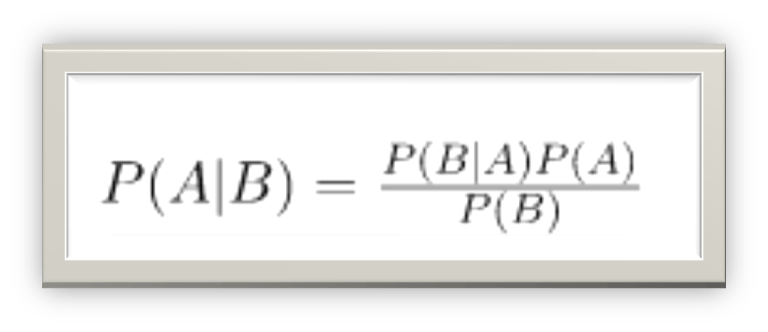
Naive Bayes is a supervised machine learning model. So, it needs both the data and the label for training the model. Naive Bayes classifiers are a collection of classification algorithms based on the Bayes Theorem.The basic assumption of Naive Bayes is that each feature makes an independent and equal contribution to the outcome.Bayes Theorem finds the probability of an event occurring given the probability of another event that has already occurred. It can be mathematically stated as:

In Naive Bayes model we assume that each feature is independent with respect to each other. Naive Bayes Classifier is used when:

• Training Data is small.
• Text Classifications is to be done.
• Small number of features are there.
• Dataset changes frequently.

In the above shown formula:

1. P(A/B)is the posterior probability of event A when event B has already occurred.
2. P(A)is the prior probability of event A.
3. P(B)is the probability of event B.
4. P(B/A)is the likelihood.

Now let us take an example of classifying a data or message to be a spam or not.

Consider spam message with label 1 and legitimate message with label 0 which can be shown as below:

Spam - 0

Legitimate – 1

Consider a dataset where X is the messages each with n features and size of the features is equal to the size of the vocabulary. There are total m messages with n features of each so the matrix can be represented as m x n size.

The probability of a message to be Legitimate given X messages can be given as:

The probability of a message to be spam given X messages can be given as:

Final prediction will be considered as maximum among y=0 and y=1.

E.g. Suppose that ,

Probability of P(y=1/X) = 0.8

Probability of P(y=0/X) = 0.2

Result = max(P(y=1/X), P(y=0/X))

Thus, in our case it is 0.8 so the message will be classified as Legitimate.

P(X/y=0) indicates in how many messages is the given word appearing.

P (Spam/” Discount”) = P (Discount / Spam) * P(Spam)

-> Where, P(Scam) = total number of spam label containing message / total number of messages in the dataset.

X is the collection of vectors so X can be given as X = (x1, x2, x3...xn). Therefore, according to Bayes theorem:

P (x1, x2, x3…. xn/y=1) = P(x1/y=1) P (x2/y=1, x1) P (x3/y=1, x1, x2) ………. P (xn/y=1, x1, x2, x3, …., xn-1)

-> Where the trailing x1, x2 and so on are the previous probabilities.

Now let us make an assumption that the probability of P(X/y) depends only on the conditional probability P(Xi/y) and not on the previous probabilities that is x1, x2, xi-1 which can be useful for real world problems. Thus, we can write it as:

P (x1, x2, x3…. xn/y=1) = P(x1/y=1) P (x2/y=1,) P (x3/y=1) ………. P (xn/y=1,)

The above assumption made is very naive so the classifier is known as Naive Bayes Classifier.

Therefore,

P(X/y=1) = πP(Xi/y=1)

So according to Bayes Theorem,

P(y=1/X) = πP(Xi/y=1) * P(y=1) / P(X)

But the denominator will be ignored therefore,

P(y=1/X) = πP(Xi/y=1) * P(y=1)

Naive Bayes for text can be given as: Probability of the word appearing in the document can be given with respect to the number of the words appearing in the dataset. Size of the vocabulary and total number of features should be same.

Inbuilt function .fit_transform( ) is used to create the vocabulary which contains the words with their respective index value and .transform( ) is used to test the new data for which the prediction has to be made.

But there is one problem with this classifier. The problem is that if newer document is given to the model for prediction then if the word given in the newer data is not available in the prebuilt vocabulary then the model will predict the probability as 0. But this is not the proper way to deal with this type of situation. So, we can use a technique named as Laplace Smoothing which says that the word appeared at least 1 time.

I hope this was an useful read! Comment your views, feedbacks and something you think this article must contain.

Thanks for reading! 😊